Approximating Pi using Python: Monte Carlo Approach
/ 4 min read
1. What is Pi?
Pi () is the ratio of a circle’s circumference to its diameter, with its value being approximately 3.1415. It is an irrational number, which means it has an infinite number of decimal places without repeating patterns. Mathematicians have computed trillions of digits of Pi; however, for most practical applications, approximations are often sufficient and more practical to use. But can we approximate the true value of Pi, in a “fast” computational way? One fascinating approach involves probability, randomness, and Monte Carlo simulations.
2. Linking probability and approximation
Monte Carlo methods are a class of algorithms that rely on probability and repeated random sampling in order to obtain an approximate numerical solution to a problem. They are typically used on numerical problems which have an unknown value that is difficult to calculate or approximate by other means - situations where deterministic algorithms are impractical or difficult to apply, or analytic solutions are difficult to find. However, this is only the case if it is possible to model the problem in terms of probability, as it relies on statistical analysis.
The Monte Carlo method is simple: you take random samples, define success and failure, and estimate the probability of an outcome based on the proportion of successful outcomes to the total number of samples.
3. How does Monte Carlo method help with approximating pi?
It is difficult to accurately measure the geometric properties of a perfect circle, namely the circumference and diameter, which are required to calculate Pi. Therefore, the Monte Carlo method may be taken advantage of, provided that the value of Pi can be expressed in terms of a probability. In this case, the underlying concept is to use geometric probability to produce an approximate value of Pi.
We need to define a problem where random samples can be used to approximate Pi, and to do that we will use geometry - a circle radius 1 within a square side length 2.
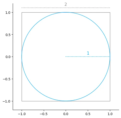
The area of the square will be
The area of the circle will be
We will randomly throw darts and assume that our aim is good enough that all darts land in the square, so what would be the probability of a dart landing inside the circle? Comparing the areas we can see the circle has an area of Pi, and the square and area of 4, so landing in the circle will have a probability of .
Now we have the probability, we can compare this to the proportion of successful trials (darts that land in the circle) to all trials (all darts thrown). That is to say if we throw enough darts, eventually darts in circle () comparted to total darts thrown () will approximate (). Rearranging for Pi we get
import random
def estimate_pi(num_points):    inside_circle = 0
    for _ in range(num_points):        x = random.uniform(-1, 1)        y = random.uniform(-1, 1)
        if x**2 + y**2 <= 1:            inside_circle += 1
    return 4 * (inside_circle / num_points)
approx_pi = estimate_pi(100_000)print(f"Estimated Pi: {approx_pi}")
Running the code once again produces a close approximation -
Estimated Pi: 3.141124. Visualising
Extending the previous code, we can plot the random points with matplotlib to visualise approximations.
import randomimport matplotlib.pyplot as plt
def estimate_pi(num_points, ax=None): inside_circle = 0 hit_x = [] hit_y = [] miss_x = [] miss_y = []
for _ in range(num_points): x = random.uniform(-1, 1) y = random.uniform(-1, 1)
if x**2 + y**2 <= 1: inside_circle += 1 hit_x.append(x) hit_y.append(y) else: miss_x.append(x) miss_y.append(y)
pi = 4 * (inside_circle / num_points)
ax.scatter(hit_x, hit_y, s=1, color="#0AF") ax.scatter(miss_x, miss_y, s=1, color="#00A") ax.set_xlim([-1.2, 1.2]) ax.set_ylim([-1.2, 1.2]) ax.set_aspect('equal', adjustable='box') ax.set_title(f'Num Points: {num_points:,}, Pi: {pi:.5f}')
return pi
test = [10_000*n for n in range(1,7)]
fig, axes = plt.subplots(2, 3, figsize=(15, 10), sharey=True)axes = axes.flatten()
for i, num_points in enumerate(test): approx_pi = estimate_pi(num_points, axes[i]) print(f"Estimated Pi: {approx_pi}")
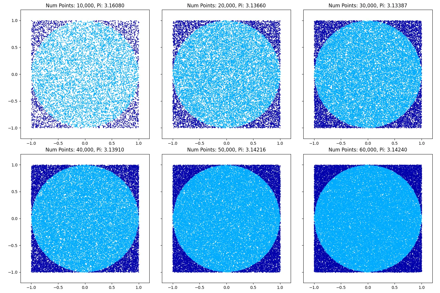
plt.tight_layout()plt.savefig('monte-carlo-pi-estimations.png')Running the code and using an increasing number of points (10k to 60k), we get closer to the true value of Pi, and the image of a circle becomes clearer. Beyond 60k points, the image becomes indistinguishable from a circle.
Past 60k I just picked some arbitrary numbers to get approximations for, up to 1B which is the max my computer could handle and still run in under 10 minutes.
| Num points | Pi | Error |
|---|---|---|
| 10k | 3.1608 | -0.0192073464 |
| 20k | 3.1366 | 0.0049926536 |
| 30k | 3.13387 | 0.0077226536 |
| 40k | 3.1391 | 0.0024926536 |
| 50k | 3.14216 | -0.0005673464 |
| 60k | 3.1424 | -0.0008073464 |
| 100k | 3.14112 | 0.0004726536 |
| 500k | 3.141176 | 0.0004166536 |
| 1M | 3.140324 | 0.0012686536 |
| 10M | 3.141186 | 0.0004066536 |
| 100M | 3.14123516 | 0.0003574936 |
| 1B | 3.141655136 | -0.0000624824 |
The approximations are clearly converging. By examining the first four digits over the last three rounds, we can confidently conclude that 3.141 are the first four digits of Pi, as they have remained consistent.